Introduction
Goal
The aim is to :
- have an understanding of the nature of ChIP-Seq data
- perform a complete analysis workflow including quality check (QC), read mapping, visualization in a genome browser and peak-calling. Use command line and open source software for each each step of the workflow and feel the complexity of the task
- have an overview of possible downstream analyses
- perform a motif analysis with online web programs
Summary
This training gives an introduction to ChIP-seq data analysis, covering the processing steps starting from the reads to the peaks. Among all possible downstream analyses, the practical aspect will focus on motif analyses. A particular emphasis will be put on deciding which downstream analyses to perform depending on the biological question.
This training does not cover all methods available today. It does not aim at bringing users to a professional NGS analyst level but provides enough information to allow biologists understand what DNA sequencing practically is and to communicate with NGS experts for more in-depth needs.
Dataset description
For this training, we will use a dataset produced by Myers et al (see on the right of the page for details on the publication) involved in the regulation of gene expression under anaerobic conditions in bacteria. We will focus on one factor: FNR.
Downloading ChIP-seq reads from NCBI
Goal: Identify the dataset corresponding to the studied article and retrieve the data (reads as FASTQ file) corresponding to one experiment and the control.
Related VIB training: Downloading NGS data from NCBI
1 - Obtaining an identifier for a chosen dataset
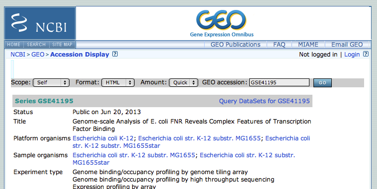
Within an article of interest, search for a sentence mentioning the deposition of the data in a database. Here, the following sentence can be found at the end of the Materials and Methods section:
"All genome-wide data from this publication have been deposited in NCBI’s Gene Expression Omnibus (GSE41195)."
We will thus use the GSE41195 identifier to retrieve the dataset from the NCBI GEO (Gene Expression Omnibus) database.
NGS datasets are (usually) made freely accessible for other scientists, by depositing these datasets into specialized databanks.
Sequence Read Archive (SRA) located in USA hosted by NCBI, and its european equivalent European Nucleotide Archive (ENA) located in England hosted by EBI both contains raw reads.
Functional genomic datasets (transcriptomics, genome-wide binding such as ChIP-seq,...) are deposited in the databases Gene Expression Omnibus (GEO) or its European equivalent ArrayExpress.
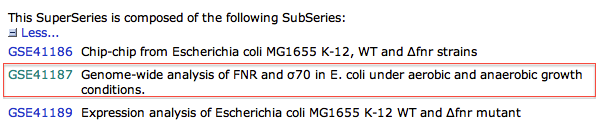
2 - Accessing GSE41195 from GEO
3 - Downloading FASTQ file from the ENA database
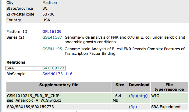
Although direct access to the SRA database at the NCBI is doable, SRA does not store the sequence FASTQ format. In practice, it's simpler (and quicker!!) to download datasets from the ENA database (European Nucleotide Archive) hosted by EBI (European Bioinformatics Institute) in UK. ENA encompasses the data from SRA.
- Go to the EBI website. Paste your SRA identifier (SRX189773) and click on the button "search"
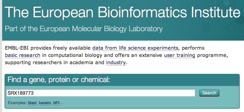
- Click on the first result. On the next page, there is a link to the FASTQ file. For efficiency, this file has already been downloaded and is available in the "data" folder (SRR576933.fastq)
To download the control dataset, we should redo the same steps starting from the GEO web page specific to the chip-seq datasets (see step 2.4) and choose anaerobic INPUT DNA.
The downloaded FASTQ file is available in the data folder (SRR576938.fastq)
At this point, you should have two FASTQ files, one for the experiment, one for the control. In which organism are you working ?
Quality control of the reads and statistics
Goal: Get some basic information on the data (read length, number of reads, global quality of dataset)
Related VIB training: Quality control of NGS data
1 - Getting the FASTQC report
Before you analyze the data, it is crucial to check the quality of the data. We will use the standard tool for checking the quality of data generated on the Illumina platform: FASTQC.
Now is the time to gather your courage and face the terminal. Don't worry, it's not as scary as it seems ! Below, the "$" sign is to indicate what you must type in the command line, but don't type the "$".
- Open the terminal and go to the course directory.
$ cd /home/bits/NGS/ChIPSeq
- First check the help page of the program to see its usage and parameters.
fastqc --help
- Launch the FASTQC program on the experiment file (SRR576933.fastq)
$ fastqc SRR576933.fastq
- Wait until the analysis is finished. Check the files output by the program.
$ ls
SRR576933_fastqc  SRR576933_fastqc.zip	SRR576933.fastq
- Access the result
$ cd SRR576933_fastqc
$ ls
fastqc_data.txt  fastqc_report.html  Icons  Images  summary.txt
- Open the HTML file fastqc_report.html in Firefox.
Analyze the result of the FASTQC program:
How many reads are present in the file ?
What is the read length ?
Is the overall quality good ?
Are there any concerns raised by the report ? If so, can you tell where the problem might come from ?
There are 3 603 544 reads of 36bp. The overall quality is good, although it drops at the last position, which is usual with Illumina sequencing, so this feature is not raising hard concerns. There are several "red lights" in the report. In particular, the per sequence GC content and the duplication level are problematic. If you check the "overrepresented sequences", you'll notice a high percentage of adapters (29% !). Ideally, we would remove these adapters (=trim) the reads, and then re-run FASTQC. In practice, we often skip this step, as these reads will anyway not be mapped. Warning: this will affect the future calculated "% of mapped read" !!
- Now do the same with the control (Input) dataset (SRR576938.fastq).
Analyze the result of the FASTQC program
There are 6 717 074 reads of 36bp. The overall quality is good, although it drops at the last position, which is usual with Illumina sequencing, so this feature is not raising hard concerns. The duplication level is high, which could be due to the high coverage. We will check this later, by visualizing the dataset in a genome browser.
2 - Organism length
Knowing your organism size is important to evaluate if your dataset has sufficient coverage to continue your analyses. For the human genome (3 Gb), we usually aim at least 10 Million reads.
- Go to the NCBI Genome website, and search for the organism Escherichia coli
- Click on the Escherichia coli str. K-12 substr. MG1655 to access statistics on this genome.
How long is the genome ?
Do both FASTQ files contain enough reads for a proper analysis ?
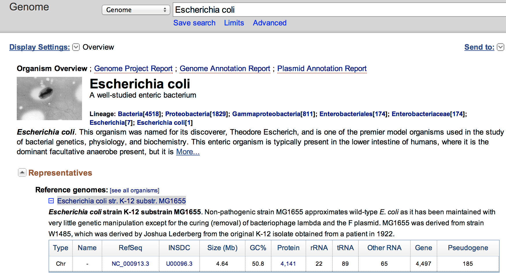
The genome is 4.64 Mbase. The files have respectively 3.6 M reads and 6.7 M reads. As we aim for 10 M for 3 Gb when working with human, the dataset here should enough reads for proper analysis.
At this point, you should be confident about the quality of the datasets, and wether it's worth following with analyzing the datasets.
Mapping the reads with Bowtie
Goal: Obtain the coordinates of each read on the reference genome.
Related VIB training: Mapping of NGS data
1 - Choosing a mapping program
There are multiple programs to perform the mapping step. For reads produced by an Illumina machine for ChIP-seq, the currently "standard" programs are BWA and Bowtie (versions 1 and 2), and STAR is getting popular. We will use Bowtie version 1.1.1 for this exercice, as this program remains effective for short reads (< 50bp).
2 - Prepare the index file
- Try out bowtie
$ bowtie-1.1.1
This prints the help of the program. However, this is a bit difficult to read ! If you need to know more about the program, it's easier to directly check the manual on the website (if it's up-to-date !)
- bowtie needs the reference genome to align each read on it. This genome needs to be in a specific format (=index) for bowtie to be able to use it. Several pre-built indexes are available to download on the bowtie webpage, but our genome is not there. You will need to make this index file.
- To make the index file, you will need the complete genome, in FASTA format. It has already been downloaded to gain time (Escherichia_coli_K12.fasta in the course folder) (The genome was downloaded from the NCBI). Note that we will not work with the lastest version (NC_000913.3) but the previous one (NC_000913.2), because the available tools for visualization have not been updated yet to the latest version. This will not affect our results.
- Build the index for bowtie
$ bowtie-1.1.1-build Escherichia_coli_K12.fasta Escherichia_coli_K12
3 - Mapping the experiment
- Let's see the parameters of bowtie before launching the mapping:
- Escherichia_coli_K12 is the name of our genome index file
- Number of mismatches for SOAP-like alignment policy (-v): to 2, which will allow two mismatches anywhere in the read, when aligning the read to the genome sequence.
- Suppress all alignments for a read if more than n reportable alignments exist (-m): to 1, which will exclude the reads that do not map uniquely to the genome.
- -q indicates the input file is in FASTQ format. SRR576933.fastq is the name of our FASTQ file.
- -3 will trim x base from the end of the read. As our last position is of low quality, we'll trim 1 base.
- -S will output the result in SAM format
- 2> SRR576933.out will output some statistics about the mapping in the file SRR576933.out
$ bowtie-1.1.1 Escherichia_coli_K12 -q SRR576933.fastq -v 2 -m 1 -3 1 -S 2> SRR576933.out > SRR576933.sam
- This should take few minutes as we work with a small genome. For the human genome, we would need either more time, or a dedicated server.
Analyze the result of the mapped reads:
Open the file SRR576933.out, which contains some statistics about the mapping. How many reads were mapped ?
$ less SRR576933.out
# reads processed: 3603544
# reads with at least one reported alignment: 2242431 (62.23%)
# reads that failed to align: 1258533 (34.92%)
# reads with alignments suppressed due to -m: 102580 (2.85%)
Reported 2242431 alignments to 1 output stream(s)
Type
q to go back.
62% of mapped reads is good, especially as we know there were adapter sequences in 29% of the reads.
4 - Mapping the control
- Repeat the steps above (step 3) for the file SRR576938.fastq.
Analyze the result of the mapped reads:
Open the file SRR576938.out. How many reads were mapped ?
$ bowtie-1.1.1 Escherichia_coli_K12 -q SRR576938.fastq -v 2 -m 1 -3 1 -S 2> SRR576938.out > SRR576938.sam
$less SRR576938.out
# reads processed: 6717074
# reads with at least one reported alignment: 6393027 (95.18%)
# reads that failed to align: 107750 (1.60%)
# reads with alignments suppressed due to -m: 216297 (3.22%)
Reported 6393027 alignments to 1 output stream(s)
95% of mapped reads is very good.
At this point, you should have two SAM files, one for the experiment, one for the control. Check the size of your files, how large are they ?
Bonus: checking two ENCODE quality metrics
Goal: This optional exercice aims at calculating the NSC and RSC ENCODE quality metrics. These metrics allow to classify the datasets (after mapping, contrary to FASTC that works on raw reads) in regards to the NSC and RSC values observed in the ENCODE datasets (see
ENCODE guidelines)
1 - PhantomPeakQualTools
Warning : this exercice is new and is tested for the first time in a classroom context. Let us know if you encounter any issue.
The SAM format correspond to large text files, that can be compressed ("zipped") into BAM format. The BAM format are usually sorted and indexed for fast access to the data it contains.
- convert the SAM file into a sorted BAM file
$ samtools-0.1.19 view -bS SRR576933.sam > SRR576933.bam
- convert the BAM file into TagAlign format, specific to the program that calculates the quality metrics
$ samtools-0.1.19 view -F 0x0204 -o - SRR576933.bam | awk 'BEGIN{OFS="\t"}{if (and($2,16) > 0) {print $3,($4-1),($4-1+length($10)),"N","1000","-"} else {print $3,($4-1),($4-1+length($10)),"N","1000","+"} }' | gzip -c > SRR576933_experiment.tagAlign.gz
- Run phantompeakqualtools
$ Rscript /usr/bin/tools/phantompeakqualtools/run_spp.R -c=SRR576933_experiment.tagAlign.gz -savp -out=SRR576933_experiment_phantompeaks
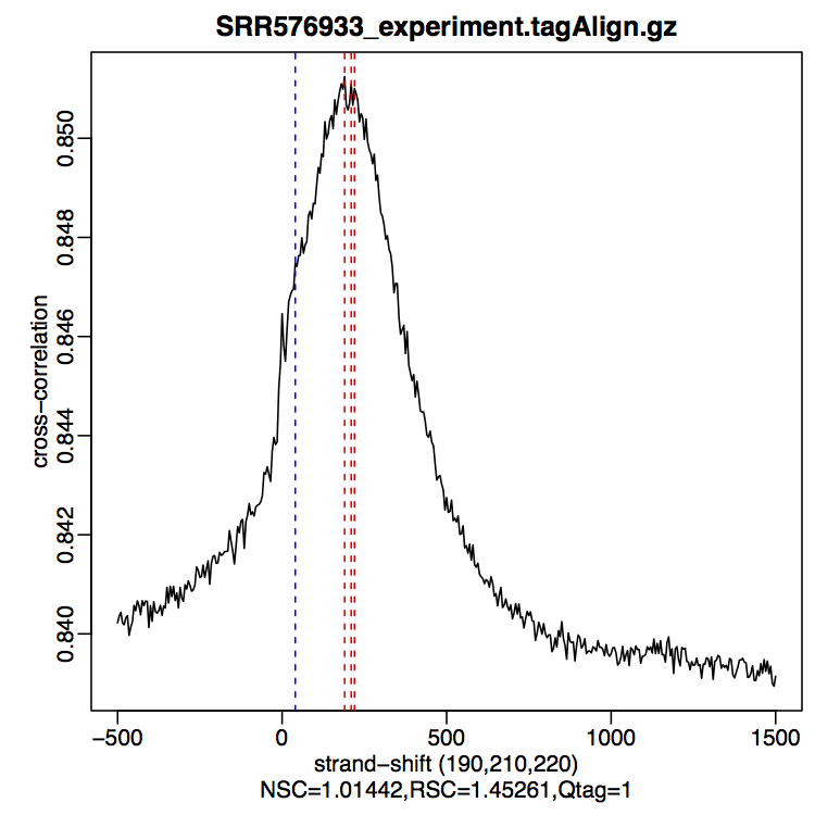
A PDF file named SRR576933_experiment.tagAlign.pdf should have been produced.
According to the ENCODE guidelines, NSC >=� 1.05 ; RSC >= �0.8 is recommended. Qtag values range from -2,-1,0,1,2
What is the quality of this dataset ?
In the PDF file, below the x-axis of the figure, are listed the NSC, RSC and Qtag values. The NSC is lower than the accepted threshold, but RSC and Qtag are good.
Warning: these values are for vertebrate, so in the context of this E. coli dataset, it is difficult to interpret these values correctly. For more details, see
Marinov et al, 2014.
At this point, you should be able to measure the ENCODE RSC and NSC metric values on a given dataset.
Peak calling with MACS
Goal: Define the peaks, i.e. the region with a high density of reads, where the studied factor was bound
1 - Choosing a peak-calling program
There are multiple programs to perform the peak-calling step. Some are more directed towards histone marks (broad peaks) while others are specific to narrow peaks (transcription factors). Here we will use MACS version 1.4.2 because it's known to produce generally good results, and it is well-maintained by the developper. A new version (MACS2) is being developped, but still in testing phase so we will not use it today.
2 - Calling the peaks
- Try out MACS
$ macs14
This prints the help of the program.
- Let's see the parameters of MACS before launching the mapping:
- ChIP-seq tag file (-t) is the name of our experiment (treatment) mapped read file SRR576933.sam
- ChIP-seq control file (-c) is the name of our input (control) mapped read file SRR576938.sam
- --format SAM indicates the input file are in SAM format. Other formats can be specified (BAM,BED...)
- --gsize Effective genome size: this is the size of the genome considered "usable" for peak calling. This value is given by the MACS developpers on their website. It is smaller than the complete genome because many regions are excluded (telomeres, highly repeated regions...). The default value is for human (2700000000.0), so we need to chnage it. As the value for E. coli is not provided, we will take the complete genome size 4639675.
- --name provides a prefix for the output files. We set this to macs14, but it could be any name.
- --bw The bandwidth is the size of the fragment extracted from the gel electrophoresis or expected from sonication. By default, this value is 300bp. Usually, this value is indicated in the Methods section of publications. In the studied publication, a sentence mentions "400bp fragments (FNR libraries)". We thus set this value to 400.
- --keep-dup specifies how MACS should treat the reads that are located at the exact same location (duplicates). The manual specifies that keeping only 1 representative of these "stacks" of reads is giving the best results.
- --bdg --single-profile will output a file in BEDGRAPH format to visualize the peak profiles in a genome browser. There will be one file for the treatment, and one for the control.
- --diag is optional and increases the running time. It tests the saturation of the dataset, and gives an idea of how many peaks are found with subsets of the initial dataset.
- &> MACS.out will output the verbosity (=information) in the file MACS.out
$ macs14 -t SRR576933.sam -c SRR576938.sam --format SAM --gsize 4639675 --name "macs14" --bw 400 --keep-dup 1 --bdg --single-profile --diag &> MACS.out
- This should take about 10 minutes, mainly because of the
--diag and the --bdg options. Without, the program runs much faster.
3 - Analyzing the MACS results
Look at the files that were created by MACS. Which files contains which information ?
$ ls -h
MACS.out
macs14_MACS_bedGraph
macs14_diag.xls
macs14_negative_peaks.xls
macs14_peaks.bed
macs14_peaks.xls
macs14_summits.bed
- MACS.out: information on MACS run.
- macs14_diag.xls: diagnostic file. Here, we see that most of the peaks (83%) are found with only 20% of the initial dataset, indicating saturation.
- macs14_negative_peaks.xls: peaks called when inverting the treatment and the control.
- macs14_peaks.bed: peak coordinates in BED format
- macs14_peaks.xls: peak coordinates with more information, to be opened with Excel
- macs14_summits.bed: location of the summit base for each peak (BED format)
How many peaks were detected by MACS ?
$ wc -l macs14_peaks.bed
109 peaks were called with these parameters. In the article, the authors found 207 peaks, by integrating the results of 3 peak-calling programs and additional ChIP-chip data.
At this point, you should have a BED file containing the peak coordinates (and two BEDGRAPH files for the treatment and the control).
Visualizing the peaks in a genome browser
1 - Choosing a genome browser
There are several options for genome browsers, divided between the local browsers (need to install the program, eg. IGV) and the online web browsers (eg. UCSC genome browser, Ensembl). We often use both types, depending on the aim and the localisation of the data.
If the data are on your computer, to prevent data transfer, it's easier to visualize the data locally (IGV). Note that if you're working on a non-model organism, the local viewer will be the only choice. If the aim is to share the results with your collaborators, view many tracks in the context of many existing annotations, then the online genome browsers are more suitable.
2 - Viewing the peaks in IGV
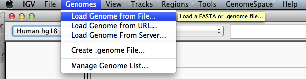
- Open IGV
$ igv
- Load the desired genome:
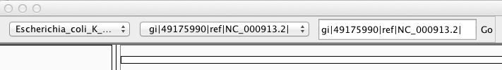
Load the Escherichia coli K12 MG1655 genome as reference
(from the fasta file Escherichia_coli_K_12_MG1655.fasta, used to build the bowtie index file)
The loaded genome appears in the top left panel:
- Unzip the bedgraph files and rename them with the extension .bedgraph, otherwise the file will not be recognized by IGV.
$ gunzip macs14_control_afterfiting_all.bdg.gz
mv macs14_control_afterfiting_all.bdg macs14_control_afterfiting_all.bedgraph
Do the same for the treatment file
- View the bedgraph files
Load the control bedgraph file
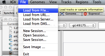
You might get a warning that the file is big. Simply click on the button
continue.
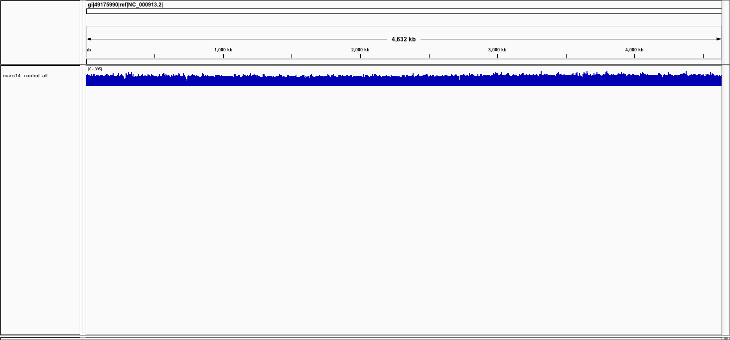
You should see the track (in blue).
Repeat this step to load the treatment bedgraph file
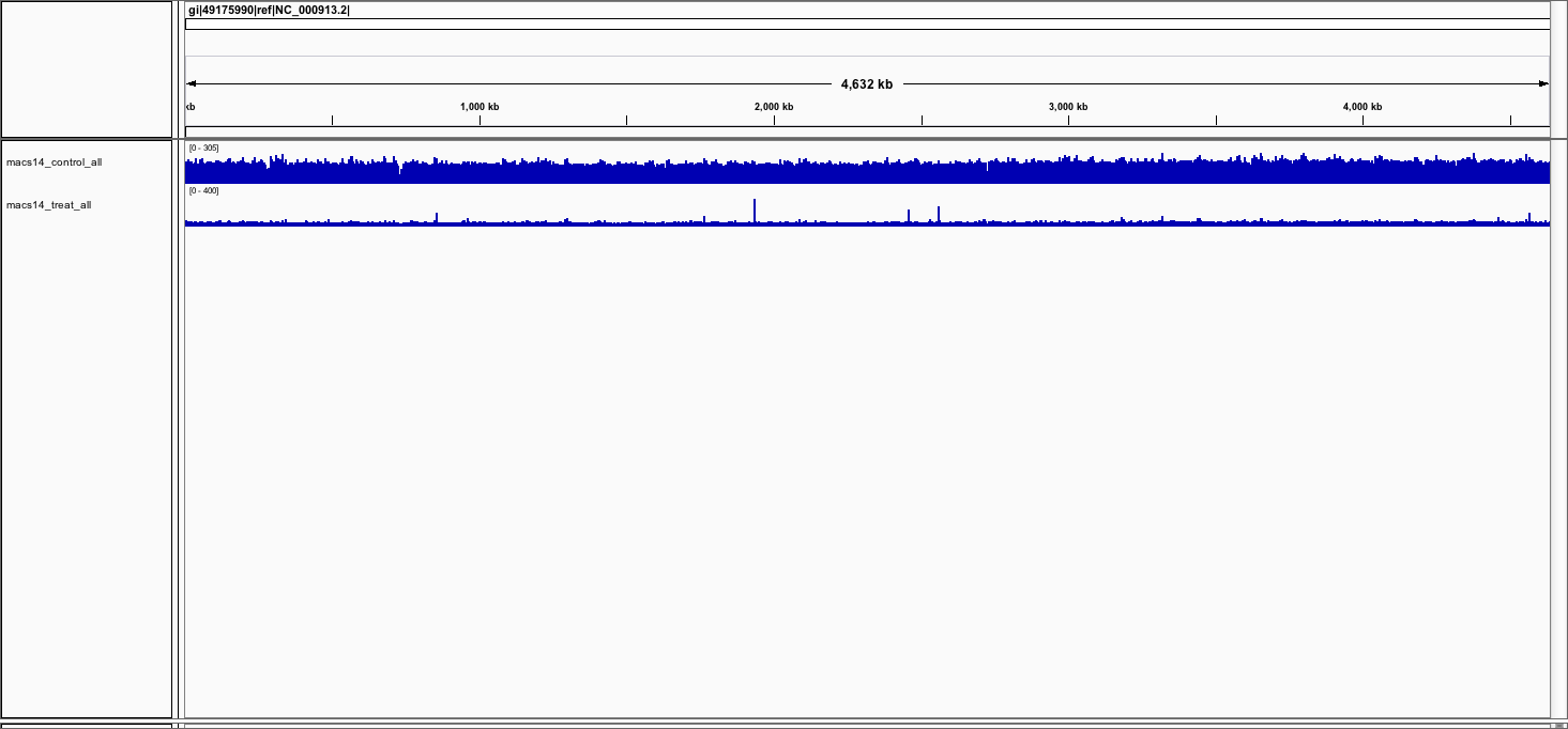
You should now see the 2 tracks (in blue).
- View the BED file containing the peak locations
Load the BED file macs14_peaks.bed
A new track with discrete positions appears at the bottom:
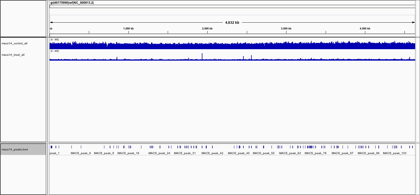
- To see the genes, load the file Escherichia_coli_K_12_MG1655.annotation.fixed.bed
At this point, you should have viewed your peaks in the genome browser. Why do the control look "bigger" than the treatment ? How could we fix this ?
Bonus: vizualisation with deeptools
Goal: This optional exercice illustrate some usage of the recent
DeepTools suite for visualization
1 - From SAM to sorted BAM
The SAM format correspond to large text files, that can be compressed ("zipped") into BAM format. The BAM format are usually sorted and indexed for fast access to the data it contains.
- convert the SAM file into a sorted BAM file
$ samtools-0.1.19 view -bS SRR576933.sam | samtools-0.1.19 sort - SRR576933_sorted
- Remove the duplicated reads
$ samtools-0.1.19 rmdup -s SRR576933_sorted.bam SRR576933_sorted_nodup.bam
from 2242431 uniquely mapped reads, it remains 1142724 reads without duplicates.
- Index the BAM file
$ samtools-0.1.19 index SRR576933_sorted_nodup.bam SRR576933_sorted_nodup.bai
2 - From BAM to scaled Bedgraph files
- bamCoverage from deepTools generates BedGraphs from BAM files
$ bamCoverage --help
- Generate a scaled BedGraph file
$ bamCoverage --bam SRR576933_sorted_nodup.bam --outFileName SRR576933_nodup.bedgraph --outFileFormat bedgraph --normalizeTo1x 4639675
Rerun all these steps for the control file. Load the two bedgraph files in IGV, make sure the two tracks are displayed with the same data range (right-click on the track, "Set Data Range...")
2152727 reads remain after removing the duplicates in the control file.
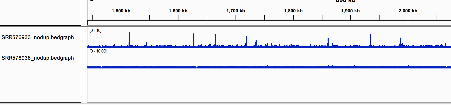
At this point, you should have viewed your treatment and control with scaled files in IGV.
Motif analysis
Goal: Define binding motif(s) for the ChIPed transcription factor and identify potential cofactors
1 - Retrieve the peak sequences corresponding to the peak coordinate file (BED)
For the motif analysis, you first need to extract the sequences corresponding the the peaks. There are several ways to do this (as usual...). If you work on a UCSC-supported organism, the easiest is to use RSAT fetch-sequences or Galaxy .
Here, we will use Bedtools, as we have the genome of our interest on our computer (Escherichia_coli_K_12_MG1655.fasta).
$ bedtools getfasta -fi Escherichia_coli_K_12_MG1655.fasta -bed macs14_peaks.bed -fo macs14_peaks.fa
Always check that the number of sequences really corresponds to the number of peaks
The idea is to count the number of lines that starts with '>' (=fasta headers)
$ grep -c '^>' macs14_peaks.fa
2 - Motif discovery with RSAT
- Open a connection to a Regulatory Sequence Analysis Tools server. You can choose between various website mirrors.
- In the left menu, click on NGS ChIP-seq and then click on peak-motifs. A new page opens, with a form
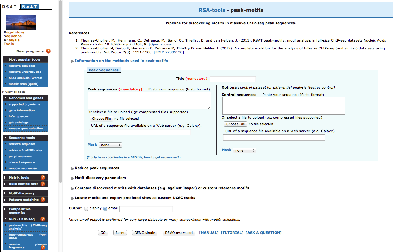
- The default peak-motifs web form only displays the essential options. There are only two
mandatory parameters.
a. The title box, which you will set as FNR Anaerobic A
b. The sequences, that you will upload from your computer, by clicking on the buttonChoose file, and select the file macs14_peaks.fa from your computer.
- We could launch the analysis like this, but we will now modify some of the advanced options in order to fine-tune the analysis according
to your data set.
- Open the "Reduce peak sequences" title, and make sure the "Cut peak sequences: +/- " option is set to 0 (we wish to analyse our full dataset)
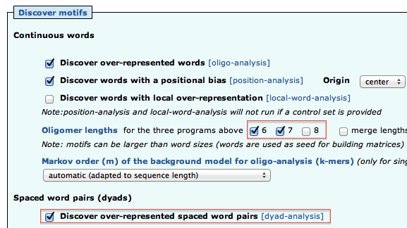
- Open the “Motif Discovery parameters” title, and check the oligomer sizes 6 and 7 (but not 8). Check "Discover over-represented spaced word pairs [dyad-analysis]"
- Under “Compare discovered motifs with databases”, uncheck "JASPAR core vertebrates" and check RegulonDB prokaryotes (2012_05) as the studied organism is the bacteria E. coli.
- You can indicate your email address in order to receive notification of the task submission and completion. This is particularly useful because the full analysis may take some time for very large datasets.
- Click “GO”. As soon as the query has been launched, you should receive an email indicating confirming the task submission, and providing a link to the future result page.
- The Web page also displays a link, You can already click on this link. The report will be progressively updated during the processing of the workflow.
Do we discover significant motifs ? Are these motifs biologically relevant? In particular, did the program discover motifs related
to FNR ?
The programs returns motifs, but many have low significance values. None of the motifs resembles any known motifs from the database RegulonDB, which is not a good sign.
Look at the top of the report (Sequence composition panel). Can you explain why the results are not so good ?
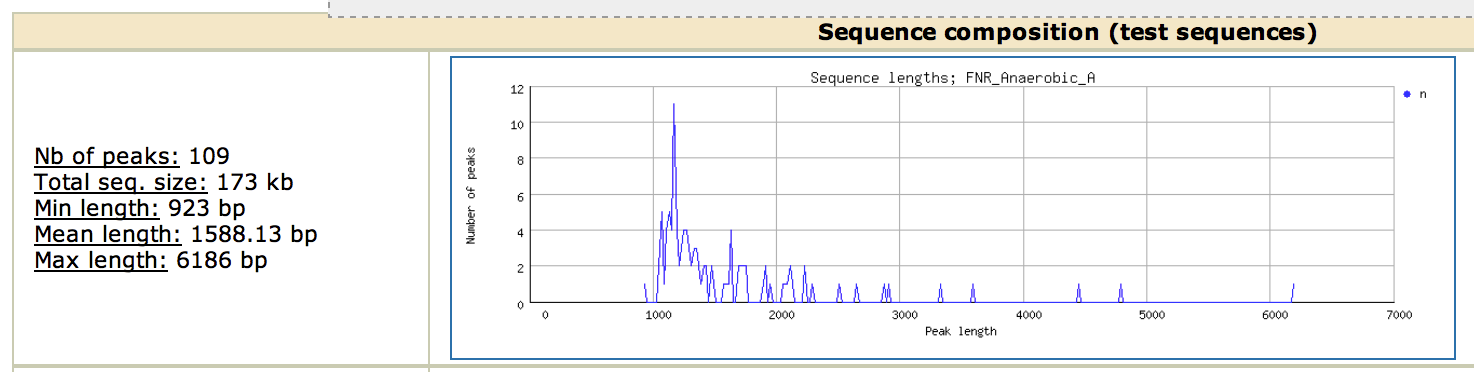
This section is extremely important, as it gives you information about your dataset. Here, we see that our 109 peaks are extremely long : a minimal length of 928bp and a mean of 1.5kb, while the fragment size was 400 bp!! Note that this is a know issue
with MACS, that tends to output large peaks. For pedagogic purposes, this step was important to show the importance of peak calling on the motif analysis step. There are different options to overcome this issue: take only the region around the summit of the peaks (often a good solution, see below) or try an alternative peak-calling program (Note that this issue is apparently resolved in the next version of MACS).
3 - Motif discovery with RSAT (short peaks)
- Restrict the dataset to the summit of the peaks +/- 100bp
$ perl -lane '$start=$F[1]-100 ; $end = $F[2]+100 ; print "$F[0]\t$start\t$end"' macs14_summits.bed > macs14_summits+-100.bed
- Extract the sequences for this BED file
$ bedtools getfasta -fi Escherichia_coli_K_12_MG1655.fasta -bed macs14_summits+-100.bed -fo macs14_summits+-100.fa
- Run RSAT peak-motifs with the same options, but choosing as input file this new dataset (macs14_summits+-100.fa)
and setting the title box to FNR Anaerobic A summit +/-100bp
This time, do we discover significant motifs ? Are these motifs biologically relevant? In particular, did the program discover motifs related
to FNR ?
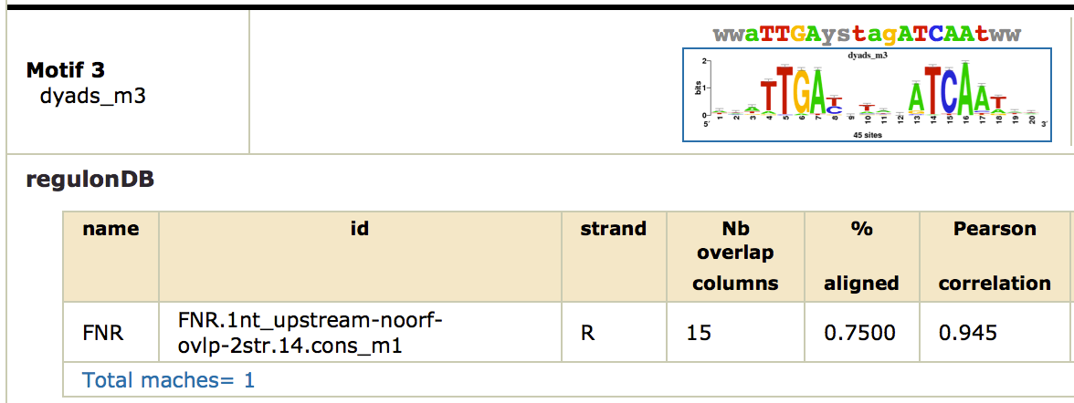
This time, we obtain a nice symmetric motif that matches the known FNR motif from RegulonDB. Click on the link
[ alignments (logos): html on the right of the found motif. You can see the alignment as a logo with the known FNR motif.
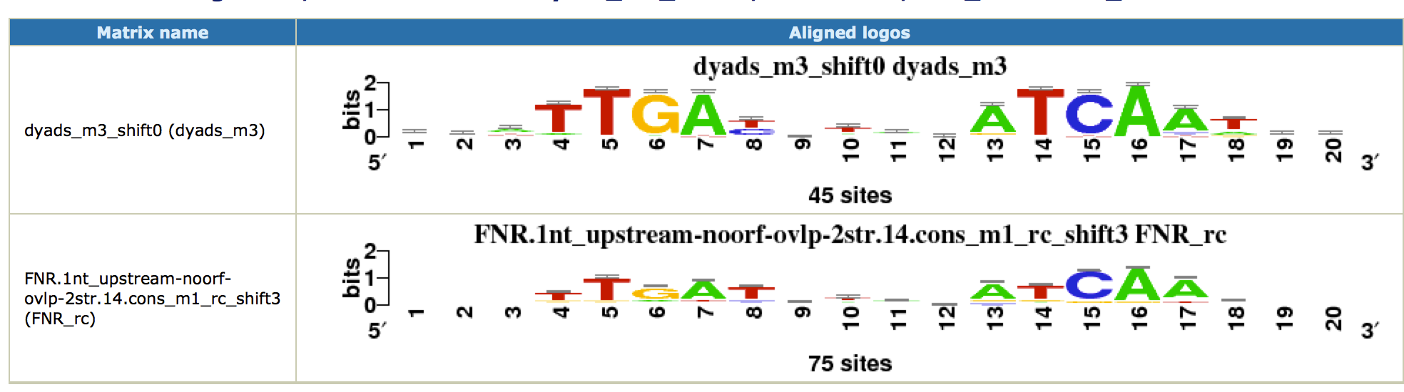
Note that this motif was only found by the
dyad-analysis
program, which highlights the importance of using several complementary algorithms for motif discovery. As there are no other factors, we did not find potential cofactors with this approach.
At this point, you should know if your motif analysis has output a motif for your ChIped TF, and if you have potential cofactors to suggest.
FAQ
How to extract peaks from the supplementary data of a publication ?
The processed peaks (BED file) is sometimes available on the GEO website, or in supplementary data. Unfortunately, most of the time, the peak coordinates are embedded into supplementary tables and thus not usable "as is".
This is the case for the studied article. To be able to use these peaks (visualize them in a genome browser, compare them with the peaks found with another program, perform downstream analyses...), you will need to (re)-create a BED file from the information available.
Here, Table S5 provides the coordinates of the summit of the peaks. The coordinates are for the same assembly as we used.
- copy/paste the first column into a new file, and save it as retained_peaks.txt
- use a PERL command (or awk if you know this language) to create a BED-formatted file. As we need start and end coordinates, we will arbitrarily take +/-50bp around the summit.
perl -lane 'print "gi|49175990|ref|NC_000913.2|\t".($F[0]-50)."\t".($F[0]+50)."\t" ' retained_peaks.txt > retained_peaks.bed
- The BED file looks like this:
gi|49175990|ref|NC_000913.2|	120	220
gi|49175990|ref|NC_000913.2|	20536	20636
gi|49175990|ref|NC_000913.2|	29565	29665
gi|49175990|ref|NC_000913.2|	34015	34115
- Depending on the available information, the command will be different.
How to obtain the annotation (=Gene) BED file for IGV?
Annotation files can be found on genome websites, NCBI FTP server, Ensembl, ... However, IGV required GFF format, or BED format, which are often not directly available.
Here, I downloaded the annotation from the UCSC Table browser as "Escherichia_coli_K_12_MG1655.annotation.bed". Then, I changed the "chr" to the name of our genome with the following PERL command:
perl -pe 's/^chr/gi\|49175990\|ref\|NC_000913.2\|/' Escherichia_coli_K_12_MG1655.annotation.bed > Escherichia_coli_K_12_MG1655.annotation.fixed.bed
This file will work directly in IGV